Chapter 5
Inventory Costing and Valuation
This chapter reviews how the cost of goods sold is calculated using various inventory cost flow assumptions. Additionally, issues related to merchandise inventory that remains on hand at the end of an accounting period are also explored.
Chapter 5 Learning Objectives
- LO1 – Calculate cost of goods sold and merchandise inventory using specific identification, first-in first-out (FIFO), and weighted average cost flow assumptions — perpetual.
- LO2 – Explain the impact on financial statements of inventory cost flows and errors.
- LO3 – Explain and calculate lower of cost and net realizable value inventory adjustments.
- LO4 – Estimate merchandise inventory using the gross profit method and the retail inventory method.
- LO5 – Explain and calculate merchandise inventory turnover.
- LO6 – Calculate cost of goods sold and merchandise inventory using specific identification, first-in first-out (FIFO), and weighted average cost flow assumptions — periodic.
Concept Self-Check
Use the following as a self-check while working through Chapter 5
- What three inventory cost flow assumptions can be used in perpetual inventory systems?
- What impact does the use of different inventory cost flow assumptions have on financial statements?
- What is the meaning of the term lower of cost and net realizable value, and how is it calculated?
- What is the effect on net income of an error in ending inventory values?
- What methods are used to estimate ending inventory?
- What ratio can be used to evaluate the liquidity of merchandise inventory?
- What inventory cost flow assumptions can be used in a periodic inventory system?
NOTE: The purpose of these questions is to prepare you for the concepts introduced in the chapter. Your goal should be to answer each of these questions as you read through the chapter. If, when you complete the chapter, you are unable to answer one or more the Concept Self-Check questions, go back through the content to find the answer(s). Solutions are not provided to these questions.
5.1 Inventory Cost Flow Assumptions
LO1 – Calculate cost of goods sold and merchandise inventory using specific identification, first in first-out (FIFO), and weighted average cost flow assumptions — perpetual.
Determining the cost of each unit of inventory, and thus the total cost of ending inventory on the balance sheet, can be challenging. Why? We know from Chapter 5 that the cost of inventory can be affected by discounts, returns, transportation costs, and shrinkage. Additionally, the purchase cost of an inventory item can be different from one purchase to the next. For example, the cost of coffee beans could be $5.00 a kilo in October and $7.00 a kilo in November. Finally, some types of inventory flow into and out of the warehouse in a specific sequence, while others do not. For example, milk would need to be managed so that the oldest milk is sold first. In contrast, a car dealership has no control over which vehicles are sold because customers make specific choices based on what is available. So how is the cost of a unit in merchandise inventory determined? There are several methods that can be used. Each method may result in a different cost, as described in the following sections.
Assume a company sells only one product and uses the perpetual inventory system. It has no beginning inventory at June 1, 2015. The company purchased five units during June as shown in Figure 5.1:
| Purchase Transaction | ||||
| Date | Number of units | Price per unit | ||
| June 1 | 1 | $1 | ||
| 5 | 1 | 2 | ||
| 7 | 1 | 3 | ||
| 21 | 1 | 4 | ||
| 28 | 1 | 5 | ||
| 5 | $15 | |||
At June 28, there are 5 units in inventory with a total cost of $15 ($1 + $2 + $3 + $4 + $5). Assume four units are sold June 30 for $10 each on account. The cost of the four units sold could be determined based on identifying the cost associated with the specific units sold. For example, a car dealership tracks the cost of each vehicle purchased and sold. Alternatively, a business that sells perishable items would want the oldest units to move out of inventory first to minimize spoilage. Finally, if large quantities of low dollar value items are in inventory, such as pencils or hammers, an average cost might be used to calculate cost of goods sold. A business may choose one of three methods to calculate cost of goods and the resulting ending inventory based on an assumed flow. These methods are: specific identification, FIFO, and weighted average, and are discussed in the next sections.
Specific Identification
Under specific identification, each inventory item that is sold is matched with its purchase cost. This method is most practical when inventory consists of relatively few, expensive items, particularly when individual units can be identified with serial numbers — for example, motor vehicles.
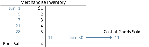
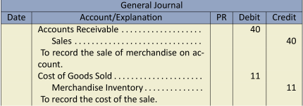
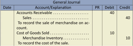
Assume the four units sold on June 30 are those purchased on June 1, 5, 7, and 28. The fourth unit purchased on June 21 remains in ending inventory. Cost of goods sold would total $11 ($1 + $2 + $3 + $5). Sales would total $40 (4 @ $10). As a result, gross profit would be $29 ($40 – 11). Ending inventory would be $4, the cost of the unit purchased on June 21.
The general ledger T-accounts for Merchandise Inventory and Cost of Goods Sold would show:
The entry to record the June 30 sale on account would be:
It is not possible to use specific identification when inventory consists of a large number of similar, inexpensive items that cannot be easily differentiated. Consequently, a method of assigning costs to inventory items based on an assumed flow of goods can be adopted. Two such generally accepted methods, known as cost flow assumptions, are discussed next.
The First-in, First-out (FIFO) Cost Flow Assumption
First-in, first-out (FIFO) assumes that the first goods purchased are the first ones sold. A FIFO cost flow assumption makes sense when inventory consists of perishable items such as groceries and other time-sensitive goods.
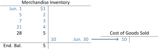
Using the information from the previous example, the first four units purchased are assumed to be the first four units sold under FIFO. The cost of the four units sold is $10 ($1 + $2 + $3 + $4). Sales still equal $40, so gross profit under FIFO is $30 ($40 – $10). The cost of the one remaining unit in ending inventory would be the cost of the fifth unit purchased ($5).
The general ledger T-accounts for Merchandise Inventory and Cost of Goods Sold as illustrated in Figure 5.3 would show:
The entry to record the sale would be:
The Weighted Average Cost Flow Assumption
A weighted average cost flow is assumed when goods purchased on different dates are mixed with each other. The weighted average cost assumption is popular in practice because it is easy to calculate. It is also suitable when inventory is held in common storage facilities — for example, when several crude oil shipments are stored in one large holding tank. To calculate a weighted average, the total cost of all purchases of a particular inventory type is divided by the number of units purchased.
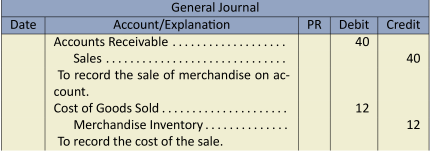
To calculate the weighted average cost in our example, the purchase prices for all five units are totaled ($1 + $2 + $3 + $4 + $5 = $15) and divided by the total number of units purchased (5). The weighted average cost for each unit is $3 ($15/5). The weighted average cost of goods sold would be $12 (4 units @ $3). Sales still equal $40 resulting in a gross profit under weighted average of $28 ($40 – $12). The cost of the one remaining unit in ending inventory is $3.
The general ledger T-accounts for Merchandise Inventory and Cost of Goods Sold are:
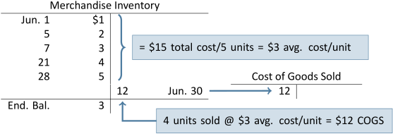
The entry to record the sale would be:
Cost Flow Assumptions: A Comprehensive Example
Recall that under the perpetual inventory system, cost of goods sold is calculated and recorded in the accounting system at the time when sales are recorded. In our simplified example, all sales occurred on June 30 after all inventory had been purchased. In reality, the purchase and sale of merchandise is continuous. To demonstrate the calculations when purchases and sales occur continuously throughout the accounting period, let’s review a more comprehensive example.
Assume the same example as above, except that sales of units occur as follows during June:
| Date | Number of Units Sold | |
| June 3 | 1 | |
| 8 | 1 | |
| 23 | 1 | |
| 29 | 1 |
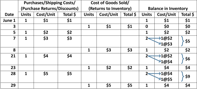
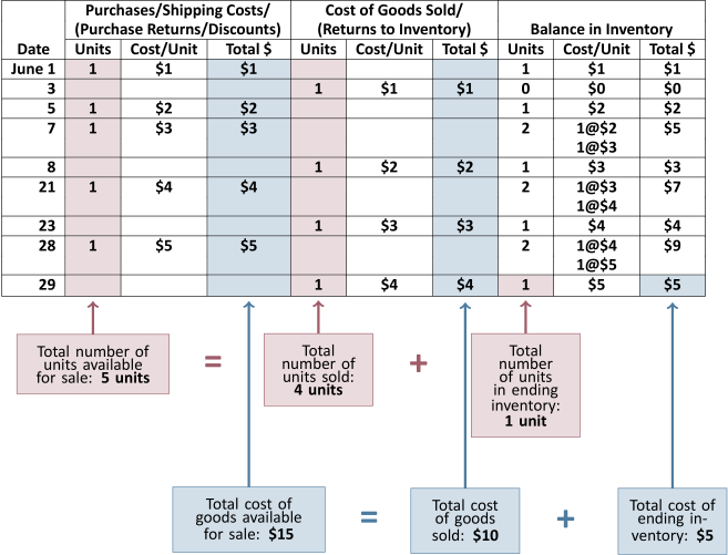
To help with the calculation of cost of goods sold, an inventory record card will be used to track the individual transactions. This card records information about purchases such as the date, number of units purchased, and purchase cost per unit. It also records cost of goods sold information: the date of sale, number of units sold, and the cost of each unit sold. Finally, the card records the balance of units on hand, the cost of each unit held, and the total cost of the units on hand. A partially-completed inventory record card is shown in Figure 5.5 below:
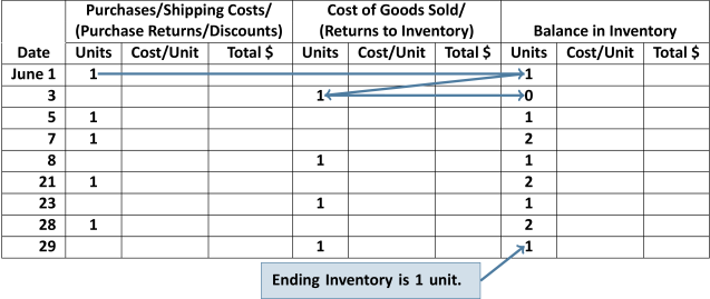
In Figure 5.5, the inventory at the end of the accounting period is one unit. This is the number of units on hand according to the accounting records. A physical inventory count must still be done, generally at the end of the fiscal year, to verify the quantities actually on hand. As discussed in Chapter 5, any discrepancies identified by the physical inventory count are adjusted for as shrinkage.
As purchases and sales are made, costs are assigned to the goods using the chosen cost flow assumption. This information is used to calculate the cost of goods sold amount for each sales transaction at the time of sale. These costs will vary depending on the inventory cost flow assumption used. As we will see in the next sections, the cost of sales may also vary depending on when sales occur.
Comprehensive Example—Specific Identification
To apply specific identification, we need information about which units were sold on each date. Assume that specific units were sold as detailed below:
| Date of Sale | Specific Units Sold | |
| June 3 | The unit sold on June 3 was purchased on June 1 | |
| 8 | The unit sold on June 8 was purchased on June 7 | |
| 23 | The unit sold on June 23 was purchased on June 5 | |
| 29 | The unit sold on June 29 was purchased on June 28 | |
Using the information above to apply specific identification, the resulting inventory record card appears in Figure 5.6:
Notice in Figure 5.7 that the number of units sold plus the units in ending inventory equals the total units that were available for sale. This will always be true regardless of which inventory cost flow method is used:
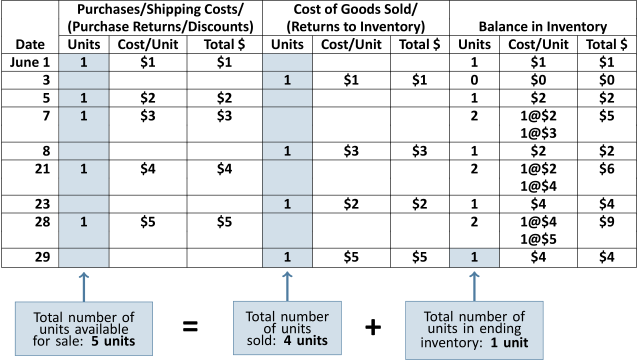
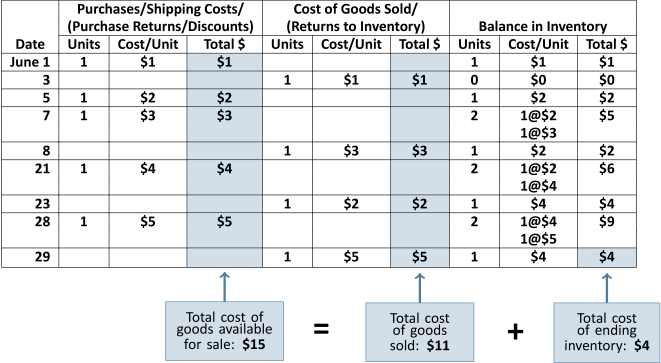
Figure 5.8 highlights the relationship in which total cost of goods sold plus total cost of ending inventory equals total cost of goods available for sale. This relationship will always be true for each of specific identification, FIFO, and weighted average.
Comprehensive Example—FIFO (Perpetual)
Using the same information, we now apply the FIFO cost flow assumption as shown in Figure 5.9:
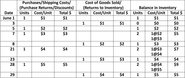
When calculating the cost of the units sold in FIFO, the oldest unit in inventory will always be the first unit removed. For example, in Figure 5.9, on June 8, one unit is sold when the previous balance in inventory consisted of 2 units: 1 unit purchased on June 5 that cost $2 and 1 unit purchased on June 7 that cost $3. Because the unit costing $2 was in inventory first (before the June 7 unit costing $3), the cost assigned to the unit sold on June 8 is $2. Under FIFO, the first units into inventory are assumed to be the first units removed from inventory when calculating cost of goods sold. Therefore, under FIFO, ending inventory will always be the most recent units purchased. In Figure 5.9, there is one unit in ending inventory and it is assigned the $5 cost of the most recent purchase which was made on June 28.
The information in Figure 5.9 is repeated in Figure 5.10 to reinforce that goods available for sale equals the sum of goods sold and ending inventory:
Comprehensive Example—Weighted Average (Perpetual)
The inventory record card transactions using weighted average costing are detailed in Figure 5.11. For consistency, all weighted average calculations will be rounded to two decimal places. When a perpetual inventory system is used, the weighted average is calculated each time a purchase is made. For example, after the June 7 purchase, the balance in inventory is 2 units with a total cost of $5.00 (1 unit at $2.00 + 1 unit at $3.00) resulting in an average cost per unit of $2.50 ($5.00 ![]() 2 units = $2.50). When a sale occurs, the cost of the sale is based on the most recent average cost per unit. For example, the cost of the sale on June 3 uses the $1.00 average cost per unit from June 1 while the cost of the sale on June 8 uses the $2.50 average cost per unit from June 7:
2 units = $2.50). When a sale occurs, the cost of the sale is based on the most recent average cost per unit. For example, the cost of the sale on June 3 uses the $1.00 average cost per unit from June 1 while the cost of the sale on June 8 uses the $2.50 average cost per unit from June 7:
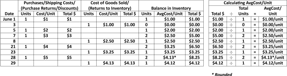
A common error made by students when applying weighted average occurs when the unit costs are rounded. For example, on June 28, the average cost per unit is rounded to $4.13 ($8.25 ![]() 2 units = $4.125/unit rounded to $4.13). On June 29, the cost of the unit sold is $4.13, the June 28 average cost per unit. Care must be taken to recognize that the total remaining balance in inventory after the June 29 sale is $4.12, calculated as the June 28 ending inventory total dollar amount of $8.25 less the June 29 total cost of goods sold of $4.13. Students will often incorrectly use the average cost per unit, in this case $4.13, to calculate the ending inventory balance. Remember that the cost of goods sold plus the balance in inventory must equal the goods available for sale as highlighted in Figure 5.12:
2 units = $4.125/unit rounded to $4.13). On June 29, the cost of the unit sold is $4.13, the June 28 average cost per unit. Care must be taken to recognize that the total remaining balance in inventory after the June 29 sale is $4.12, calculated as the June 28 ending inventory total dollar amount of $8.25 less the June 29 total cost of goods sold of $4.13. Students will often incorrectly use the average cost per unit, in this case $4.13, to calculate the ending inventory balance. Remember that the cost of goods sold plus the balance in inventory must equal the goods available for sale as highlighted in Figure 5.12:
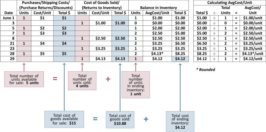
Figure 5.13 compares the results of the three cost flow methods. Goods available for sale, units sold, and units in ending inventory are the same regardless of which method is used. Because each cost flow method allocates the cost of goods available for sale in a particular way, the cost of goods sold and ending inventory values are different for each method.
| Total Cost | Total | Total | ||||
| of Goods | Units | Total Cost | Total | Total Cost | Units in | |
| Cost Flow | Available | Available | of Goods | Units | of Ending | Ending |
| Assumption | for Sale | for Sale | Sold | Sold | Inventory | Inventory |
| Specific Identification | $15.00 | 5 | 11.00 | 4 | 4.00 | 1 |
| FIFO | 15.00 | 5 | 10.00 | 4 | 5.00 | 1 |
| Weighted Average | 15.00 | 5 | 10.88 | 4 | 4.12 | 1 |
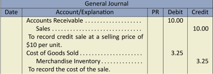
Journal Entries
We now know that the information in the inventory record is used to prepare the journal entries in the general journal. For example, the credit sale on June 23 using weighted average costing would be recorded as follows (refer to Figure 5.13):
Perpetual inventory incorporates an internal control feature that is lost under the periodic inventory method. Losses resulting from theft and error can easily be determined when the actual quantity of goods on hand is counted and compared with the quantities shown in the inventory records as being on hand. It may seem that this advantage is offset by the time and expense required to continuously update inventory records, particularly where there are thousands of different items of various sizes on hand. However, computerization makes this record keeping easier and less expensive because the inventory accounting system can be tied in to the sales system so that inventory is updated whenever a sale is recorded.
Inventory Record Card
In a company such as a large drugstore or hardware chain, inventory consists of thousands of different products. For businesses that carry large volumes of many inventory types, the general ledger merchandise inventory account contains only summarized transactions of the purchases and sales. The detailed transactions for each type of inventory would be recorded in the underlying inventory record cards. The inventory record card is an example of a subsidiary ledger, more commonly called a subledger. The merchandise inventory subledger provides a detailed listing of type, amount, and total cost of all types of inventory held at a particular point in time. The sum of the balances on each inventory record card in the subledger would always equal the ending amount recorded in the Merchandise Inventory general ledger account. So a subledger contains the detail for each product in inventory while the general ledger account shows only a summary. In this way, the general ledger information is streamlined while allowing for detail to be available through the subledger. There are other types of subledgers: the accounts receivable subledger and the accounts payable subledger. These will be introduced in a subsequent chapter.
5.2 Financial Statement Impact of Different Inventory Cost Flows
LO2 – Explain the impact of inventory cost flows and errors.
When purchase costs are increasing, as in a period of inflation (or decreasing, as in a period of deflation), each cost flow assumption results in a different value for cost of goods sold and the resulting ending inventory, gross profit, and net income.
Using information from the preceding comprehensive example, the effects of each cost flow assumption on net income and ending inventory are shown in Figure 5.14.
| Spec. | Wtd. | |||||||
| Ident. | FIFO | Avg. | ||||||
| Sales | $ | 40.00 | $ | 40.00 | $ | 40.00 | ||
| Cost of goods sold | 11.00 | 10.00 | 10.88 | |||||
| Gross profit and net income | $ | 29.00 | $ | 30.00 | $ | 29.12 | ||
| Ending inventory (on the balance sheet) | $ | 4.00 | $ | 5.00 | $ | 4.12 | ||
FIFO maximizes net income and ending inventory amounts when costs are rising. FIFO minimizes net income and ending inventory amounts when purchase costs are decreasing.
Because different cost flow assumptions can affect the financial statements, GAAP requires that the assumption adopted by a company be disclosed in its financial statements (full disclosure principle). Additionally, GAAP requires that once a method is adopted, it be used every accounting period thereafter (consistency principle) unless there is a justifiable reason to change. A business that has a variety of inventory items may choose a different cost flow assumption for each item. For example, Walmart might use weighted average to account for its sporting goods items and specific identification for each of its various major appliances.
Effect of Inventory Errors on the Financial Statements
There are two components necessary to determine the inventory value disclosed on a corporation’s balance sheet. The first component involves calculating the quantity of inventory on hand at the end of an accounting period by performing a physical inventory count. The second requirement involves assigning the most appropriate cost to this quantity of inventory.
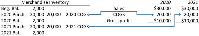
An error in calculating either the quantity or the cost of ending inventory will misstate reported income for two time periods. Assume merchandise inventory at December 31, 2019, 2020, and 2021 was reported as $2,000 and that merchandise purchases during each of 2020 and 2021 were $20,000. There were no other expenditures. Assume further that sales each year amounted to $30,000 with cost of goods sold of $20,000 resulting in gross profit of $10,000. These transactions are summarized below:
Assume now that ending inventory was misstated at December 31, 2020. Instead of the $2,000 that was reported, the correct value should have been $1,000. The effect of this error was to understate cost of goods sold on the income statement — cost of goods sold should have been $21,000 in 2020 as shown below instead of $20,000 as originally reported above. Because of the 2020 error, the 2021 beginning inventory was incorrectly reported above as $2,000 and should have been $1,000 as shown below. This caused the 2021 gross profit to be understated by $1,000 — cost of goods sold in 2021 should have been $19,000 as illustrated below but was originally reported above as $20,000:
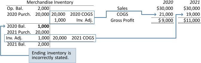
As can be seen, income is misstated in both 2020 and 2021 because cost of goods sold in both years is affected by the adjustment to ending inventory needed at the end of 2020 and 2021. The opposite effects occur when inventory is understated at the end of an accounting period.
An error in ending inventory is offset in the next year because one year’s ending inventory becomes the next year’s opening inventory. This process can be illustrated by comparing gross profits for 2020 and 2021 in the above example. The sum of both years’ gross profits is the same.
| Overstated | Correct | ||
| Inventory | Inventory | ||
| Gross profit for 2020 | $10,000 | $ 9,000 | |
| Gross profit for 2021 | 10,000 | 11,000 | |
|
Total |
$20,000 | $20,000 |
5.3 Lower of Cost and Net Realizable Value (LCNRV)
LO3 – Explain and calculate lower of cost and net realizable value inventory adjustments.
In addition to the adjusting entry to record the shrinkage of merchandise inventory, there is an additional adjusting entry to be considered at the end of the accounting period when calculating cost of goods sold and ending inventory values for the financial statements. Generally accepted accounting principles require that inventory be valued at the lesser amount of its laid-down cost and the amount for which it can likely be sold — its net realizable value (NRV). This concept is known as the lower of cost and net realizable value, or LCNRV. Note that the laid-down cost includes the invoice price of the goods (less any purchase discounts) plus transportation in, insurance while in transit, and any other expenditure made by the purchaser to get the merchandise to the place of business and ready for sale.
As an example, a change in consumer demand may mean that inventories become obsolete and need to be reduced in value below the purchase cost. This often occurs in the electronics industry as new and more popular products are introduced.
The lower of cost and net realizable value can be applied to individual inventory items or groups of similar items, as shown in Figure 5.15 below:
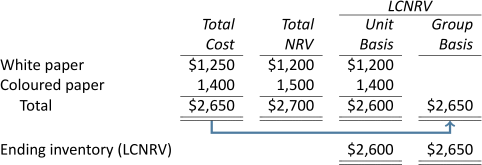
Depending on the calculation used, the valuation of ending inventory will be either $2,600 or $2,650. Under the unit basis, the lower of cost and net realizable value is selected for each item: $1,200 for white paper and $1,400 for coloured paper, for a total LCNRV of $2,600. Because the LCNRV is lower than cost, an adjusting entry must be recorded as follows:
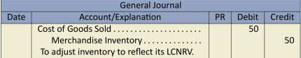
The purpose of the adjusting entry is to ensure that inventory is not overstated on the balance sheet and that income is not overstated on the income statement.
If white paper and coloured paper are considered a similar group, the calculations in Figure 5.15 above show they have a combined cost of $2,650 and a combined net realizable value of $2,700. LCNRV would therefore be $2,650. In this case, the cost is equal to the LCNRV so no adjusting entry would be required if applying LCNRV on a group basis.
5.4 Estimating the Balance in Merchandise Inventory
LO4 – Estimate merchandise inventory using the gross profit method and the retail inventory method.
A physical inventory count determines the quantity of items on hand. When costs are assigned to these items and these individual costs are added, a total inventory amount is calculated. Is this dollar amount correct? Should it be larger? How can one tell if the physical count is accurate? Being able to estimate this amount provides a check on the reasonableness of the physical count and valuation.
The two methods used to estimate the inventory dollar amount are the gross profit method and the retail inventory method. Both methods are based on a calculation of the gross profit percentage in the income statement. Assume the following information:
| Sales | $15,000 | 100% | |||
| Cost of Goods Sold: | |||||
|
Opening Inventory |
$ 4,000 | ||||
|
Purchases |
12,000 | ||||
|
Cost of Goods Available for Sale |
16,000 | ||||
|
Less: Ending Inventory |
(6,000) | ||||
| Cost of Goods Sold | 10,000 | 67% | |||
| Gross Profit | $ 5,000 | 33% |
The gross profit percentage, rounded to the nearest whole percent, is 33% ($5,000/15,000). This means that for each dollar of sales, an average of $.33 is left to cover other expenses after deducting cost of goods sold.
Estimating ending inventory requires an understanding of the relationship of ending inventory with cost of goods sold. Review the following cost of goods sold calculations:
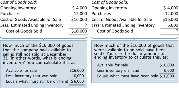
The sum of cost of goods sold and ending inventory is always equal to cost of goods available for sale. Knowing any two of these amounts enables the third amount to be calculated. Understanding this relationship is the key to estimating inventory using either the gross profit or retail inventory methods, discussed below.
Gross Profit Method
The gross profit method of estimating ending inventory assumes that the percentage of gross profit on sales remains approximately the same from period to period. Therefore, if the gross profit percentage is known, the dollar amount of ending inventory can be estimated. First, gross profit is estimated by applying the gross profit percentage to sales. From this, cost of goods sold can be derived, namely the difference between sales and gross profit. Cost of goods available for sale can be determined from the accounting records (opening inventory + purchases). The difference between cost of goods available for sale and cost of goods sold is the estimated value of ending inventory.
To demonstrate, assume that Pete’s Products Ltd. has an average gross profit percentage of 40%. If opening inventory at January 1, 2019 was $200, sales for the six months ended June 30, 2019 were $2,000, and inventory purchased during the six months ended June 30, 2019 was $1,100, the cost of goods sold and ending inventory can be estimated as follows:
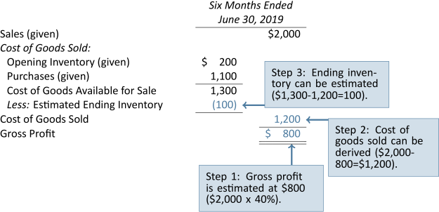
The estimated ending inventory at June 30 must be $100—the difference between the cost of goods available for sale and cost of goods sold.
The gross profit method of estimating inventory is useful in situations when goods have been stolen or destroyed by fire or when it is not cost-effective to make a physical inventory count.
Retail Inventory Method
The retail inventory method is another way to estimate cost of goods sold and ending inventory. It can be used when items are consistently valued at a known percentage of cost, known as a mark-up. A mark-up is the ratio of retail value (or selling price) to cost. For example, if an inventory item had a retail value of $12 and a cost of $10, then it was marked up to 120% (12/10 x 100). Mark-ups are commonly used in clothing stores.
To apply the retail inventory method using the mark-up percentage, the cost of goods available for sale is first converted to its retail value (the selling price). To do this, the mark-up (ratio of retail to cost) must be known. Assume the same information as above for Pete’s Products Ltd., except that now every item in the store is marked up to 160% of its purchase price. That is, if an item is purchased for $100, it is sold for $160. Based on this, opening inventory, purchases, and cost of goods available can be restated at retail. Cost of goods sold can then be valued at retail, meaning that it will equal sales for the period. From this, ending inventory at retail can be determined and then converted back to cost using the mark-up. These steps are illustrated below:
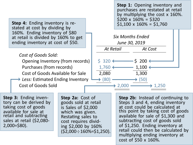
The retail inventory method of estimating ending inventory is easy to calculate and produces a relatively accurate cost of ending inventory, provided that no change in the average mark-up has occurred during the period.
5.5 Appendix A: Ratio Analysis—Merchandise Inventory Turnover
LO5 – Explain and calculate merchandise inventory turnover.
To help determine how quickly a company is able to sell its inventory, the merchandise inventory turnover can be calculated as:
| Cost of Goods Sold | Average Merchandise Inventory |
The average merchandise inventory is the beginning inventory plus the ending inventory divided by two. For example, assume Company A had cost of goods sold of $3,000; beginning merchandise inventory of $500; and ending inventory of $700. The merchandise inventory turnover would be 5, calculated as:
| Cost of Goods Sold | Average Merchandise Inventory | |
| $3,000 | (($500+$700)/2) |
The ‘5’ means that Company A sold its inventory 5 times during the year. In contrast, assume Company B had cost of goods sold of $3,000; beginning merchandise inventory of $1,000; and ending inventory of $1,400. The merchandise inventory turnover would be 2.50 calculated as:
| Cost of Goods Sold | Average Merchandise Inventory | |
| $3,000 | (($1,000+$1,400)/2) |
The ‘2.5’ means that Company B sold its inventory 2.5 times during the year which is much slower than Company A. The faster a business sells its inventory, the better, because high turnover positively affects liquidity. Liquidity is the ability to convert assets, such as merchandise inventory, into cash. Therefore, Company A’s merchandise turnover is more favourable than Company B’s.
5.6 Appendix B: Inventory Cost Flow Assumptions Under the Periodic System
LO6 – Calculate cost of goods sold and merchandise inventory using specific identification, first-in first-out (FIFO), and weighted average cost flow assumptions periodic.
Recall, that the periodic inventory system does not maintain detailed records to calculate cost of goods sold each time a sale is made. Rather, when a sale is made, the following entry is made:
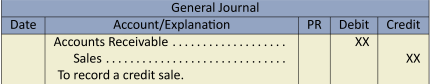
No entry is made to record cost of goods sold and to reduce Merchandise Inventory, as is done under the perpetual inventory system. Instead, all purchases are expenses and recorded in the general ledger account “Purchases.” A physical inventory count is conducted at year-end. An amount for ending inventory is calculated based on this count and the valuation of the items in inventory, and cost of goods sold is calculated in the income statement based on this total amount. The income statement format is:
| Sales | $10,000 | ||
| Cost of Goods Sold: | |||
|
Opening Inventory |
$ 1,000 | ||
|
Purchases |
5,000 | ||
|
Goods Available for Sale |
6,000 | ||
|
Less: Ending Inventory |
(2,000) | ||
| Cost of Goods Sold | 4,000 | ||
| Gross Profit | $6,000 |
Even under the periodic inventory system, however, inventory cost flow assumptions need to be made (specific identification, FIFO, weighted average) when purchase prices change over time, as in a period of inflation. Further, different inventory cost flow assumptions produce different cost of goods sold and ending inventory values, just as they did under the perpetual inventory system. These effects have been explained earlier in this chapter. Under the periodic inventory system, cost of goods sold and ending inventory values are determined as if the sales for the period all take place at the end of the period. These calculations were demonstrated in our earliest example in this chapter.
Our original example using units assumed there was no opening inventory at June 1, 2015 and that purchases were made as follows.
| Purchase Transaction | ||||
| Date | Number of units | Price per unit | ||
| June 1 | 1 | $1 | ||
| 5 | 1 | 2 | ||
| 7 | 1 | 3 | ||
| 21 | 1 | 4 | ||
| 28 | 1 | 5 | ||
| 5 | $15 | |||
When recorded in the general ledger T-account “Purchases” (an income statement account), these transactions would be recorded as follows.
| Purchases | No. 570 | ||
| Jun. 1 | $1 | ||
| 5 | 2 | ||
| 7 | 3 | ||
| 21 | 4 | ||
| 28 | 5 | ||
Sales of four units are all assumed to take place on June 30. Ending inventory would then be counted at the end of the day on June 30. One unit should be on hand. It would be valued as follows under the various inventory cost flow assumptions, as discussed in the first part of the chapter:
| Specific identification | $4 |
| FIFO | 5 |
| Weighted average | 3 |
These values would be used to calculate cost of goods sold and gross profit on the income statement, as shown in Figure 5.16 below:
| Spec. | Wtd. | ||||
| Ident. | FIFO | Avg. | |||
| Sales | $40 | $40 | $40 | ||
| Cost of Goods Sold: | |||||
|
Opening Inventory |
-0- | -0- | -0- | ||
|
Purchases |
15 | 15 | 15 | ||
|
Goods Available for Sale |
15 | 15 | 15 | ||
|
Less: Ending Inventory |
(4) | (5) | (3) | ||
| Cost of Goods Sold | 11 | 10 | 12 | ||
| Gross Profit and Net Income | $29 | $30 | $28 | ||
| Ending Inventory (Balance Sheet) | $ 4 | $ 5 | $ 3 |
Note that these results are the same as those calculated using the perpetual inventory method and assuming all sales take place on June 30 using specific identification (Figure 5.2), FIFO (Figure 5.3), and weighted average (Figure 5.4) cost flow assumptions, respectively.
As discussed, the ending inventory amount will be recorded in the accounting records when the income statement accounts are closed to the Income Summary at the end of the year. The amount of the closing entry for ending inventory is obtained from the income statement. Using the example above and assuming no other revenue or expense items, the closing entry to adjust ending inventory to actual under each inventory cost flow assumption would be as follows.
| Specific | Weighted | ||||
| Identification | FIFO | Average | |||
| Merchandise Inventory (ending) | 4 | 5 | 3 | ||
| Sales | 40 | 40 | 40 | ||
|
Income Summary |
44 | 45 | 43 | ||
| To close all income statement accounts with credit | |||||
| balances to the Income Summary and record | |||||
| ending inventory balance. |
Summary of Chapter 5 Learning Objectives
Below, you will find each of the Learning Objectives covered in Chapter 5. Additionally, there is a brief summary that highlights the important elements you learned about for each corresponding objective:
LO1 – Calculate cost of goods sold and merchandise inventory using specific identification, first-in first-out (FIFO), and weighted average cost flow assumptions—perpetual.
Cost of goods available for sale must be allocated between cost of goods sold and ending inventory using a cost flow assumption. Specific identification allocates cost to units sold by using the actual cost of the specific unit sold. FIFO (first-in first-out) allocates cost to units sold by assuming the units sold were the oldest units in inventory. Weighted average allocates cost to units sold by calculating a weighted average cost per unit at the time of sale.
LO2 – Explain the impact on financial statements of inventory cost flows and errors.
As purchase prices change, particular inventory methods will assign different cost of goods sold and resulting ending inventory to the financial statements. Specific identification achieves the exact matching of revenues and costs while weighted average accomplishes an averaging of price changes, or smoothing. The use of FIFO results in the current cost of inventory appearing on the balance sheet in ending inventory. The cost flow method in use must be disclosed in the notes to the financial statements and be applied consistently from period to period. An error in ending inventory in one period impacts the balance sheet (inventory and equity) and the income statement (COGS and net income) for that accounting period and the next. However, inventory errors in one period reverse themselves in the next.
LO3 – Explain and calculate lower of cost and net realizable value inventory adjustments.
Inventory must be evaluated, at minimum, each accounting period to determine whether the net realizable value (NRV) is lower than cost, known as the lower of cost and net realizable value (LCNRV) of inventory. An adjustment is made if the NRV is lower than cost. LCNRV can be applied to groups of similar items or by item.
LO4 – Estimate merchandise inventory using the gross profit method and the retail inventory method.
Estimating inventory using the gross profit method requires that estimated cost of goods sold be calculated by, first, multiplying net sales by the gross profit ratio. Estimated ending inventory at cost is then arrived at by taking goods available for sale at cost less the estimated cost of goods sold. To apply the retail inventory method, three calculations are required:
- retail value of goods available for sale less retail value of net sales equals retail value of ending inventory,
- goods available for sale at cost divided by retail value of goods available for sale equals cost to retail ratio, and
- retail value of ending inventory multiplied by the cost to retail ratio equals estimated cost of ending inventory.
LO5 – Explain and calculate merchandise inventory turnover.
The merchandise turnover is a liquidity ratio that measures how quickly inventory is sold. It is calculated as: COGS/Average Merchandise Inventory. Average merchandise inventory is the beginning inventory balance plus the ending inventory balance divided by two.
LO6 – Calculate cost of goods sold and merchandise inventory using specific identification, first-in first-out (FIFO), and weighted average cost flow assumptions—periodic.
Periodic systems assign cost of goods available for sale to cost of goods sold and ending inventory at the end of the accounting period. Specific identification and FIFO give identical results in each of periodic and perpetual. The weighted average cost, periodic, will differ from its perpetual counterpart because in periodic, the average cost per unit is calculated at the end of the accounting period based on total goods that were available for sale.
Review Questions
After reading through Chapter 5, take some time to review the questions below. These questions can be used as part of a discussion with other members of your class, or they can be used for your own self-assessment as you prepare for your graded assessments.
- Explain the importance of maintaining appropriate inventory levels for
- management; and
- investors and creditors.
- What aspects of accounting for inventory on financial statements would be of interest to accountants?
- What is meant by the laid-down cost of inventory?
- How does a flow of goods differ from a flow of costs? Do generally accepted accounting principles require that the flow of costs be similar to the movement of goods? Explain.
- What two factors are considered when costing merchandise for financial statement purposes? Which of these factors is most difficult to determine? Why?
- Why is consistency in inventory valuation necessary? Does the application of the consistency principle preclude a change from weighted average to FIFO? Explain.
- The ending inventory of CBCA Inc. is overstated by $5,000 at December 31, 2018. What is the effect on 2018 net income? What is the effect on 2019 net income assuming that no other inventory errors have occurred during 2019?
- When should inventory be valued at less than cost?
- What is the primary reason for the use of the LCNRV method of inventory valuation? What does the term net realisable value mean?
- When inventory is valued at LCNRV, what does cost refer to?
- What inventory cost flow assumptions are permissible under GAAP?
- Why is estimating inventory useful?
- How does the estimation of ending inventory differ between the gross profit method and the retail inventory method? Use examples to illustrate.
- When is the use of the gross profit method particularly useful?
- Does the retail inventory method assume any particular inventory cost flow assumption?
Exercises
The questions below have been included to provide you with the opportunity to practice what you have learned. These questions are supplemental – they are not a requirement for the course. If you are struggling with any of the questions, however, it is strongly recommended that you go back and review the content or connect with the instructor for additional support.
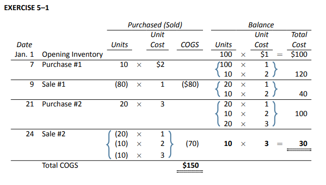
Laplante Inc. uses the perpetual inventory system. The following transactions took place during January 2021.
| Unit | ||||
| Date | Units | Cost | ||
| Jan. 1 | Opening Inventory | 100 | $1 | |
| 7 | Purchase #1 | 10 | 2 | |
| 9 | Sale #1 | 80 | ||
| 21 | Purchase #2 | 20 | 3 | |
| 24 | Sale #2 | 40 |
Using the table below, calculate cost of goods sold for the January 9 and 24 sales, and ending inventory using the FIFO cost flow assumption.
| Purchased (Sold) | Balance | |||||||||||
| Unit | Unit | Total | ||||||||||
| Date | Units | Cost | COGS | Units | Cost | Cost | ||||||
| Jan. 1 | Opening Inventory | 100 | $1 | = | $100 | |||||||
| 7 | Purchase #1 | |||||||||||
| 9 | Sale #1 | |||||||||||
| 21 | Purchase #2 | |||||||||||
| 24 | Sale #2 | |||||||||||
Click Here to View Solution
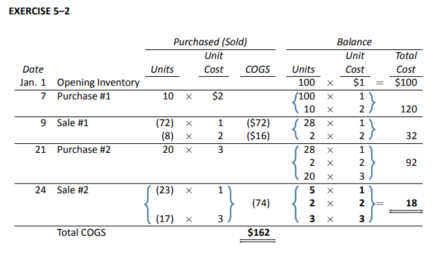
Using the information from EXERCISE 5–1, calculate the cost of goods sold for the January 9 and 24 sales, and ending inventory using the Specific Identification cost flow assumption. Assume that:
- on January 9, the specific units sold were 72 units from opening inventory and 8 units from the January 7 purchase and
- the specific units sold on January 24 were 23 units from opening inventory and 17 units from the January 21 purchase.
Click Here to View Solution
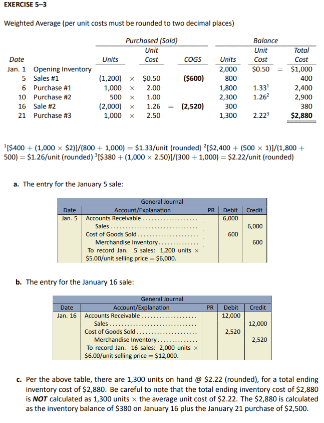
ABBA uses the weighted average inventory cost flow assumption under the perpetual inventory system. The following transactions took place in January 2018.
| Unit | |||
| Selling | |||
| Price/ | |||
| Date | Units | Cost | |
| Jan. 1 | Opening Inventory | 2,000 | $0.50 |
| 5 | Sale #1 | 1,200 | 5.00 |
| 6 | Purchase #1 | 1,000 | 2.00 |
| 10 | Purchase #2 | 500 | 1.00 |
| 16 | Sale #2 | 2,000 | 6.00 |
| 21 | Purchase #3 | 1,000 | 2.50 |
All sales are made on account. Round all per unit costs to two decimal places.
- Record the journal entry for the January 5 sale. Show calculations for cost of goods sold.
- Record the journal entry for the January 16 sale. Show calculations for cost of goods sold.
- Calculate ending inventory in units, cost per unit, and total cost.
Click Here to View Solution
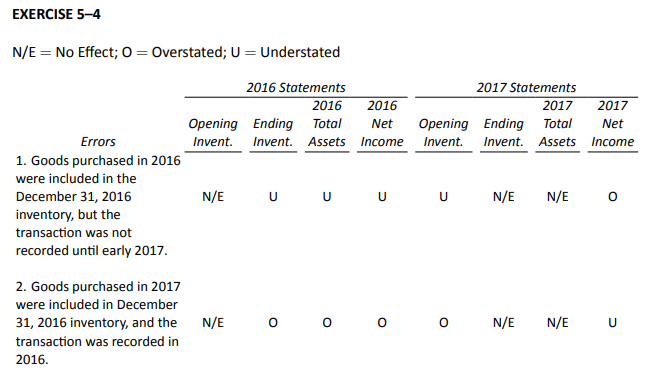
Listed below are four common accounting errors.
| 2016 Statements | 2017 Statements | ||||||||||||||
| 2016 | 2016 | 2017 | 2017 | ||||||||||||
| Opening | Ending | Total | Net | Opening | Ending | Total | Net | ||||||||
| Errors | Invent. | Invent. | Assets | Income | Invent. | Invent. | Assets | Income | |||||||
| 1. Goods purchased in 2016 | |||||||||||||||
| were included in the | |||||||||||||||
| December 31, 2016 | N/E | ||||||||||||||
| inventory, but the | |||||||||||||||
| transaction was not | |||||||||||||||
| recorded until early 2017. | |||||||||||||||
| 2. Goods purchased in 2017 | |||||||||||||||
| were included in December | |||||||||||||||
| 31, 2016 inventory, and the | N/E | ||||||||||||||
| transaction was recorded in | |||||||||||||||
| 2016. | |||||||||||||||
Use N/E (No Effect), O (Overstated), or U (Understated) to indicate the effect of each error on the company’s financial statements for the years ended December 31, 2016 and December 31, 2017. The opening inventory for the 2016 statements is done.
Click Here to View Solution
Partial income statements of Lilydale Products Inc. are reproduced below:
| 2021 | 2022 | 2023 | |||
| Sales | $30,000 | $40,000 | $50,000 | ||
| Cost of Goods Sold | 20,000 | 23,000 | 25,000 | ||
| Gross Profit | $10,000 | $17,000 | $25,000 |
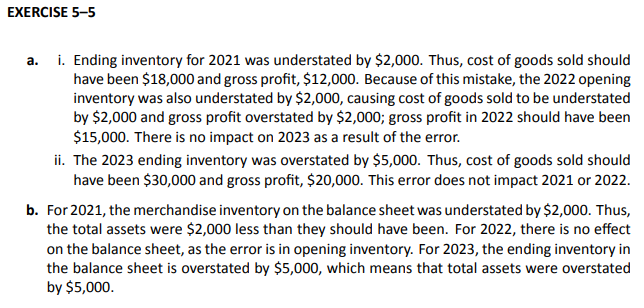
- Calculate the impact of the two errors listed below on the gross profit calculated for the three years:
- The 2021 ending inventory was understated by $2,000.
- The 2023 ending inventory was overstated by $5,000.
- What is the impact of these errors on Total Assets?
Click Here to View Solution
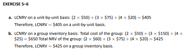
Erndale Products Ltd. has the following items in inventory at year-end:
| Item | Units | Cost/Unit | NRV/Unit | |||
| X | 2 | $50 | $60 | |||
| Y | 3 | 150 | 75 | |||
| Z | 4 | 25 | 20 |
Calculate the cost of ending inventory using LCNRV on
- A unit-by-unit basis
- A group inventory basis.
Click Here to View Solution
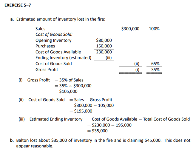
Windy City Insurance Ltd. has received a fire-loss claim of $45,000 from Balton Corp. A fire destroyed Balton’s inventory on May 25, 2015. Balton has an average gross profit of 35%. You have obtained the following information:
| Inventory, May 1, 2015 | $
80,000 |
| Purchases, May 1 – May 25 | 150,000 |
| Sales, May 1 – May 25 | 300,000 |
- Calculate the estimated amount of inventory lost in the fire.
- How reasonable is Balton’s claim?
Click Here to View Solution
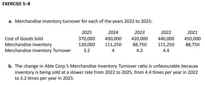
The following account balances for Cost of Goods Sold and Merchandise Inventory were extracted from Able Corp.’s accounting records:
| 2025 | 2024 | 2023 | 2022 | 2021 | |||||
| Cost of Goods Sold | 370,000 | 400,000 | 420,000 | 440,000 | 450,000 | ||||
| Merchandise Inventory | 120,000 | 111,250 | 88,750 | 111,250 | 88,750 |
- Calculate the Merchandise Inventory Turnover for each of the years 2022 to 2025.
- Is the change in Able Corp.’s Merchandise Inventory Turnover ratio favourable or unfavourable? Explain.
Click Here to View Solution
Problems
The problems that have been included in this section are more complex. They are intended to offer students the opportunity to apply what they have learned. Although these Practice Problems are optional (not for grades), they can help students better prepare for the assignment in Module 5. It is recommended that students review any relevant sections that they struggled with in answering these problems.
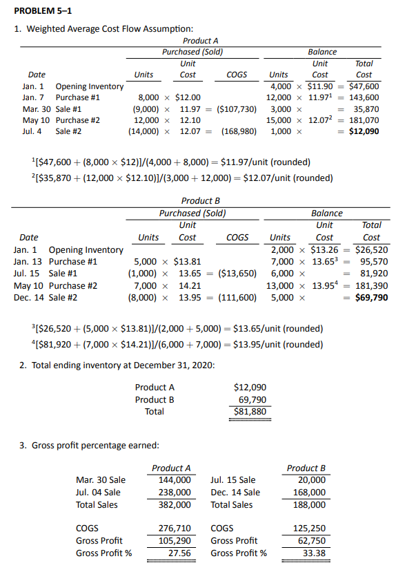
Southern Cross Company Limited made the following purchases and sales of Products A and B during the year ended December 31, 2020:
| Product A | ||||
| Unit Cost/ | ||||
| Units | Selling Price | |||
| Jan. 07 | Purchase #1 | 8,000 | $12.00 | |
| Mar. 30 | Sale #1 | 9,000 | 16.00 | |
| May 10 | Purchase #2 | 12,000 | 12.10 | |
| Jul. 04 | Sale #2 | 14,000 | 17.00 | |
| Product B | ||||
| Unit Cost/ | ||||
| Units | Selling Price | |||
| Jan. 13 | Purchase #1 | 5,000 | $13.81 | |
| Jul. 15 | Sale #1 | 1,000 | 20.00 | |
| Oct. 23 | Purchase #2 | 7,000 | 14.21 | |
| Dec. 14 | Sale #2 | 8,000 | 21.00 | |
Opening inventory at January 1 amounted to 4,000 units at $11.90 per unit for Product A and 2,000 units at $13.26 per unit for Product B.
- Prepare inventory record cards for Products A and B for the year using the weighted average inventory cost flow assumption.
- Calculate total cost of ending inventory at December 31, 2020.
- Calculate the gross profit percentage earned on the sale of
- Product A in 2020 and
- Product B in 2020.
Click Here to View Solution
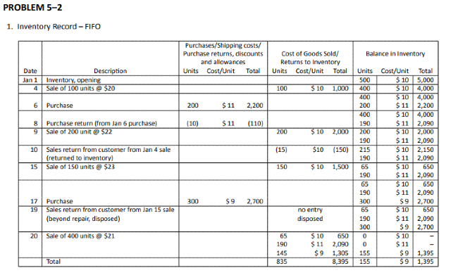
Below are various inventory related transactions:
| Jan 1 | Inventory, opening | 500 units | @ | $10 | = | $5,000 |
| 4 | Sale | 100 units | @ | $20 | = | 2,000 |
| 6 | Purchase | 200 units | @ | $11 | = | 2,200 |
| 8 | Purchase return (from Jan 6 purchase) | (10) units | @ | $11 | = | (110) |
| 9 | Sale | 200 units | @ | $22 | = | 4,400 |
| 10 | Sales return from customer from Jan 4 sale (returned to inventory) | (15) units | @ | $22 | = | (330) |
| 15 | Sale | 150 units | @ | $23 | = | 3,450 |
| 17 | Purchase | 300 units | @ | $9 | = | 2,700 |
| 19 | Sales return from customer from Jan 15 sale (beyond repair, disposed) | (2) units | $23 | = | (46) | |
| 20 | Sale | 400 units | @ | $21 | = | 2,100 |
- Complete an inventory record card (schedule) the same as the example shown in Figure 6.9 of the text and with totals at the bottom. Assume that the FIFO method was used.
- Calculate the gross profit and the gross profit percentage.
- What is the ending inventory balance at January 20, 2016?
Click Here to View Solution
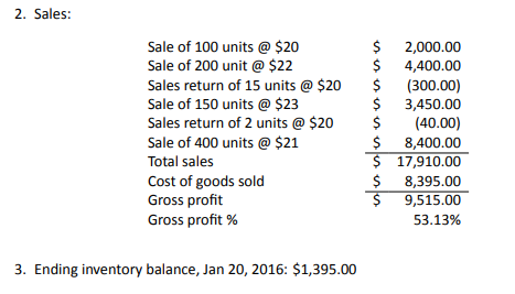
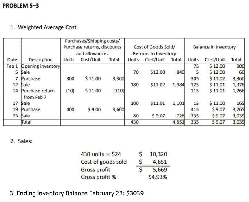
Below are various inventory related transactions:
Purchases:
| Feb 1 | Opening inventory | 75 units @ $12 |
| Feb 7 | Purchase | 300 units @ $11 |
| Feb 14 | Purchase return from Feb 7 | 10 units @ $11 |
| Feb 19 | Purchase | 400 units @ $9 |
Sales Price: $24.00
Units Sold:
| Feb 5 | 70 units |
| Feb 12 | 180 units |
| Feb 17 | 100 units |
| Feb 23 | 80 units |
- Complete an inventory record card (schedule) the same as the example shown in Figure 6.9 of the text and with totals at the bottom. Assume that a weighted average cost method was used. Round unit costs to the nearest two decimals.
- Calculate the gross profit and the gross profit percentage.
- What is the ending inventory balance at February 23, 2016?
Click Here to View Solution
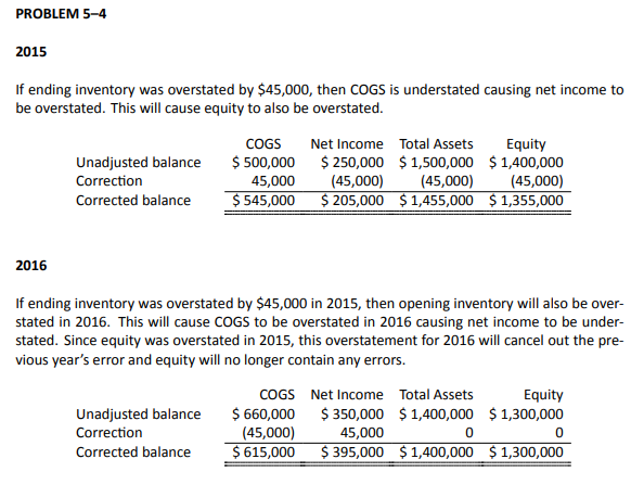
The following table shows the following financial data for AAA Ltd. for the year ended December 31, 2016:
| Financial Data | ||||||
| For the year ended December 31, 2016 | ||||||
| 2015 | 2016 | |||||
| Cost of goods sold | $ | 500,000 | $ | 660,000 | ||
| Net income | 250,000 | 350,000 | ||||
| Total assets | 1,500,000 | 1,400,000 | ||||
| Equity | 1,400,000 | 1,300,000 | ||||
The following errors were made:
The inventory count for 2015 was overstated by $45,000.
Calculate the corrected cost of goods sold, net income, total assets and equity for 2015 and 2016.
Click Here to View Solution
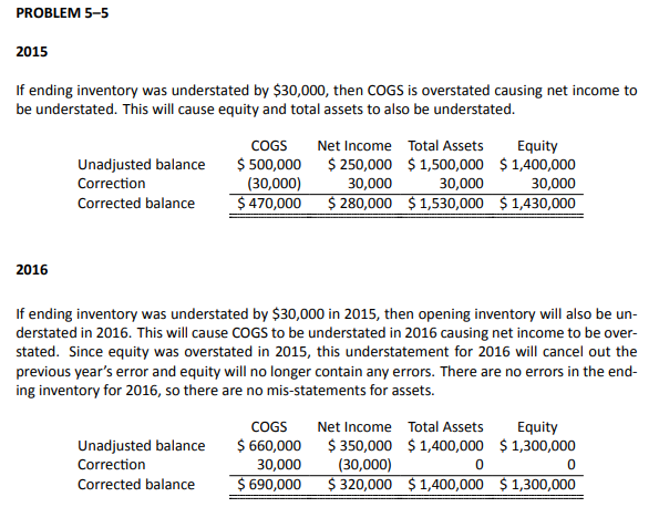
Using the data from PROBLEM 5–4, the following table shows the following financial data for AAA Ltd. for the year ended December 31, 2016:
| Financial Data | ||||||
| For the year ended December 31, 2016 | ||||||
| 2015 | 2016 | |||||
| Cost of goods sold | $ | 500,000 | $ | 660,000 | ||
| Net income | 250,000 | 350,000 | ||||
| Total assets | 1,500,000 | 1,400,000 | ||||
| Equity | 1,400,000 | 1,300,000 | ||||
The following errors were made:
The inventory count for 2015 was understated by $30,000.
Calculate the corrected cost of goods sold, net income, total assets and equity for 2015 and 2016.
Click Here to View Solution
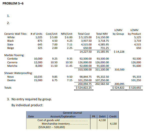
Below are the inventory details for Almac Flooring Ltd.:
| Ceramic Wall Tiles: | # of Units | Cost/Unit | NRV/Unit |
|
White |
1,025 | 5.00 | 6.00 |
|
Black |
875 | 4.50 | 4.25 |
|
Slate |
645 | 7.00 | 7.11 |
|
Beige |
325 | 2.00 | 2.25 |
| Marble Flooring: | |||
|
Cordoba |
10,000 | 9.25 | 9.35 |
|
Carrerra |
12,000 | 10.50 | 10.50 |
|
Maricha |
8,000 | 11.50 | 11.45 |
| Shower Waterproofing: | |||
|
Novo |
10,035 | 9.85 | 9.50 |
|
Deetra |
15,000 | 6.75 | 7.15 |
- Calculate the LCNRV for each group.
- Calculate the LCNRV for each individual product.
- Prepare the adjusting entries if any for parts (1) and (2).
Click Here to View Solution
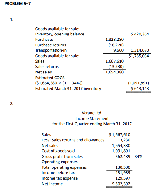
Varane Ltd. is required to submit an interim financial statement to their bank as part of the line-of-credit monitoring process. Below is information regarding their first quarter business for 2017:
| Ending inventory from the previous year | $420,364 |
| Purchases | 1,323,280 |
| Purchase returns | 18,270 |
| Transportation-in | 9,660 |
| Freight-out | 2,300 |
| Sales | 1,667,610 |
| Sales returns | 13,230 |
| Operating expenses | 130,500 |
| 3-year rolling average gross profit | 34% |
| Income tax rate | 30% |
Transportation-In should be included in inventory while Freight-Out should not be included.
- Prepare a schedule of calculations to estimate the company’s ending inventory at the end of the quarter using the gross profit method.
- Prepare a multiple-step income statement for the first quarter ending March 31, 2017.
Click Here to View Solution
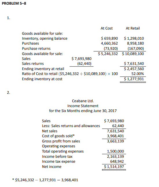
Ceabane Ltd. is required to submit an interim financial statement to their creditors. Below is information regarding their first six months for 2017:
| At Cost | At Retail | |
| Ending inventory from the previous year | $659,890 | $1,298,010 |
| Purchases | 4,660,362 | 8,958,180 |
| Purchase returns | 73,920 | 167,090 |
| Sales | 7,693,980 | |
| Sales returns | 62,440 | |
| Additional information: | ||
| Operating expenses | $1,500,000 | |
| Income tax rate | 30% |
- Prepare a schedule of calculations to estimate the company’s ending inventory at the end of the quarter using the retail inventory method.
- Prepare a multiple-step income statement for the first six months ending June 30, 2017.
Click Here to View Solution
Partial income statements of Schneider Products Inc. are reproduced below:
| 2016 | 2017 | ||
| Sales | $50,000 | $50,000 | |
| Cost of Goods Sold | 20,000 | 23,000 | |
| Gross Profit | $30,000 | $27,000 |
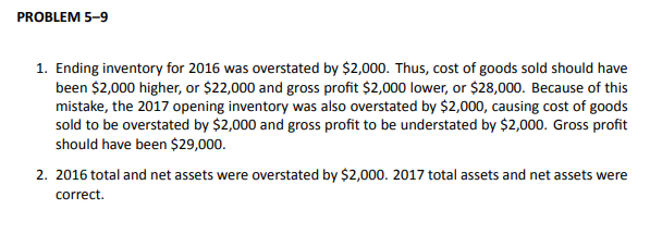
The 2016 ending inventory was overstated by $2,000 during the physical count. The 2017 physical inventory count was done properly.
- Calculate the impact of this error on the gross profit calculated for 2016 and 2017.
- What is the impact of this error on total assets at the end of 2016 and 2017? Net assets?
Click Here to View Solution
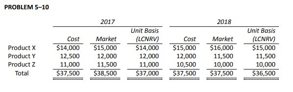
| 2017 | 2018 | ||||||||||
| Unit Basis | Unit Basis | ||||||||||
| Cost | Market | (LCNRV) | Cost | Market | (LCNRV) | ||||||
| Product X | $14,000 | $15,000 | ? | $15,000 | $16,000 | ? | |||||
| Product Y | 12,500 | 12,000 | ? | 12,000 | 11,500 | ? | |||||
| Product Z | 11,000 | 11,500 | ? | 10,500 | 10,000 | ? | |||||
|
Total |
? | ? | ? | ? | ? | ? | |||||
If Reflex values its inventory using LCNRV/unit basis, complete the 2017 and 2018 cost, net realizable value, and LCNRV calculations.
Click Here to View Solution